By Ken Steif & Michael Fichman
This post discusses some of our recent experiments with spatial real estate data. These analytics are discussed in an economics of gentrification framework. Specifically, some of Dr. Steif’s ideas regarding the supply-side conditions necessary for the wave of gentrification to move across space and time.
Introduction
The human brain is astute at detecting patterns; and so are machines – so long as they are well-trained by their human architects.
The “Supervised Learning’ process is straightforward. Feed a machine learning algorithm thousands of labeled dog and cat pictures and train it to understand the probability that a new picture is either a dog or cat.
Predictions made without labeled data or ‘Unsupervised Learning’, is far more challenging. By not knowing the outcome ahead of time, we must make inferences about the underlying system based solely on our own experience. What’s worse, there is no way to validate predictions.
Neighborhood classification is a great example of a really hard unsupervised learning task. This from Professor George Galster:
“Urban social scientists have treated ‘neighbourhood’ in much the same way as courts of law have treated pornography: as a term that is hard to define precisely, but everyone knows it when they see it.”
One creative approach for classifying neighborhood boundaries is to crowdsource the process by averaging the boundaries drawn by many community members.
There are only two of us at Urban Spatial, so crowdsourcing is out, besides we prefer an approach that is generalizable to a variety of places.
The motivation for this post is to discuss the technical and theoretical reasons for clustering home sale observations into bounded units as a way of understanding the space/time dynamics of gentrification.
The next section presents a theory of gentrification and the section to follow discusses why clustering is important for addressing this theory.
Gentrification as a motivation for clustering
Imagine two neighborhoods: Neighborhood A is surrounded on all sides with water, while Neighborhood B is surrounded on all sides by square miles of undeveloped land. What happens when housing demand faucet is turned on in both of these neighborhoods?
Our hypothesis is that prices in Neighborhood A skyrocket because there is no room to sprawl out and because the development costs (both real and regulatory) required to absorb the new demand is incredibly high. Conversely, prices in Neighborhood B do not rise as fast as new demand is absorbed by development on the hinterland.
Think San Francisco vs. Houston. In economic parlance, the former city is “supply inelastic”, meaning there is no more room to develop.
How does this apply to gentrification?
Typically, if a city neighborhood is supply inelastic or supply constrained, it is because NIMBY forces or zoning regulations are preventing development.
What happens however, when demand increases in a neighborhood which is surrounded by other neighborhoods that gentrifiers do not want to locate in?
Given a surge of new demand, the result should be the same as if that outlying neighborhood was a body of water – gentrifiers refuse to inhabit the next neighborhood over and thus prices increase because the supply of gentrifiable housing is inelastic.
This suggests a tradeoff: If a neighborhood has an inelastic supply of gentrifiable housing, we should expect price increases in the face of new demand. Conversely, if the supply is elastic and high prices are free to expand outward across space, we should observe steady house prices.
Let’s test this theory on two areas in Philadelphia.
The two submarkets on either side of Girard Avenue (Figure 1), north of Philadelphia’s downtown, provide a useful example of an inelastic supply of gentrifiable housing. Here, prices in the submarket to the south have been unable to flow north of Girard Avenue. The result has been steadily increasing prices in the submarket to the south.
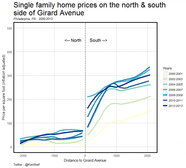
Figure 1: Prices on either side of Girard Avenue 2000-2013
Conversely, in a neighborhood just south of Philadelphia’s downtown, an entirely different spatial process is playing out (Figure 2). This area consists of two submarkets, Graduate Hospital and Point Breeze, split by Washington Avenue (in red).
Figure 2 shows that before 2006, high price home sales (defined as 5th quintile) were unable to flow south across Washington Avenue. By the close of the decade, prices creeped just below the Avenue and by 2015, nearly the entire Point Breeze neighborhood to the south was inundated with high priced home sales.
In this example, the Graduate Hospital submarket was supply elastic – meaning that when faced with rising demand, the supply of gentrifiable housing was able to expand into the next neighborhood south – Point Breeze. This sweeping wave of gentrification is evident in Figure 2.
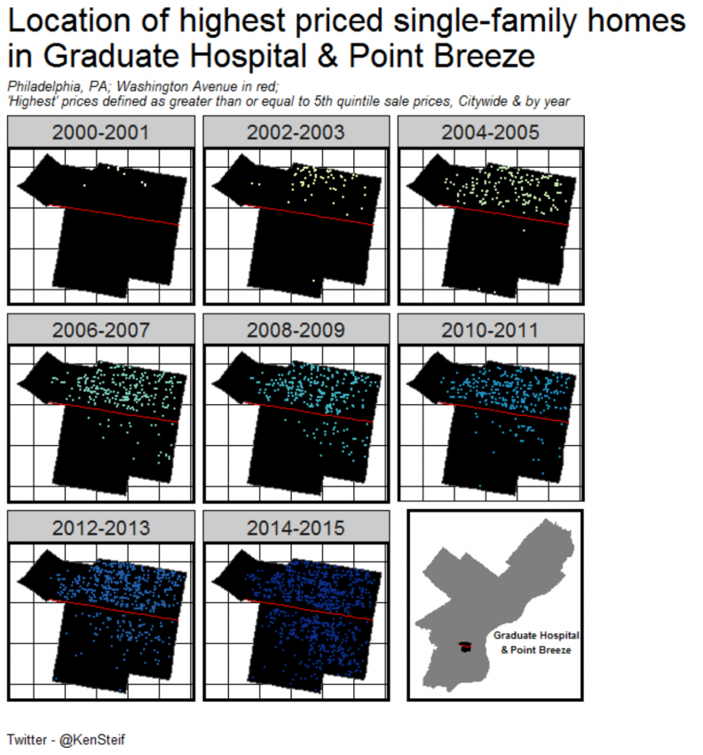
Figure 2: The wave in Graduate Hospital & Point Breeze
If our theory is correct, we should observe that prices remained steady as the supply of gentrifiable housing expanded to the south.
Indeed, this is the observable trend. Figure 3 visualizes the mean sale price per square foot over time in Graduate Hospital to the north. Note how prices increase right up until a time when the supply of gentrifiable housing expands across Washington Avenue in to Point Breeze. From here on out, prices remain relatively stable.
As we’ve discussed in previous work, the likely behavior here is that gentrifiers want to consume the amenities in and around Graduate Hospital and buying just south allows them to trade off housing costs with accessibility.
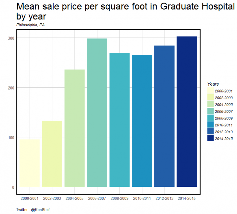
Figure 3: Prices remain steady as the wave sweeps into Point Breeze
Let’s now zoom out. How do these space/time patterns play out across the City? Figure 4 shows a gif of the highest priced home sales every year from 2001 – 2016. The data visualization illustrates the extent of gentrification over space and time emanating outward from Philadelphia’s downtown.
Figure 4: The space/time movement of high priced (5th quintile) home sales, Philadelphia
We are clearly cheating by delineating clusters in an a priori fashion as in Figure 2.
As previously discussed, what we need is an unsupervised approach and with the right algorithm in hand, we could begin to quantify some pretty useful metrics about the gentrification wave, such as where is the ‘eye of the storm’? How big is the submarket and how is it growing with respect to price? What is the trade-off between the space/time movement of clusters and changes in price?
Quantifying submarket clusters
In the examples above, we created our own clusters by subsetting sales using existing neighborhood boundaries. This is far from a ‘generalizable’ solution to the clustering challenge.
There are many clustering algorithms out there that we’ve used over the years for clustering real estate prices, but most are designed to find clusters in statistical space (x,y) not geographic space (x,y,x).
The basic premise behind any clustering algorithm is to segment objects into groups with a high degree of in-cluster homogeneity and across group heteroogeneity.
Clustering spatial data however, adds an entirely separate dimension to this otherwise simple premise. How do we balance the goal of internal similarity and external homogeneity, while accounting for variation in the manner that objects are organized in space?
In one word, the issue is one of scale, and scale is the single greatest confounding phenomena in all of spatial analysis.
Scale is problematic when analyzing arbitrary areal units; when investigating phenomena that is spatially autocorrelated; and when allocating objects to groups – such as clustering.
Most geographical techniques require that scale be parameterized in an a priori fashion and as a strictly global phenomenon (ie. spatial weights matrices).
However, scale is rarely a global phenomenon even across a single city. Take Figure 5 for example, which shows the distribution of high-priced single-family sale prices in Philadelphia and the density of those sales respectively.
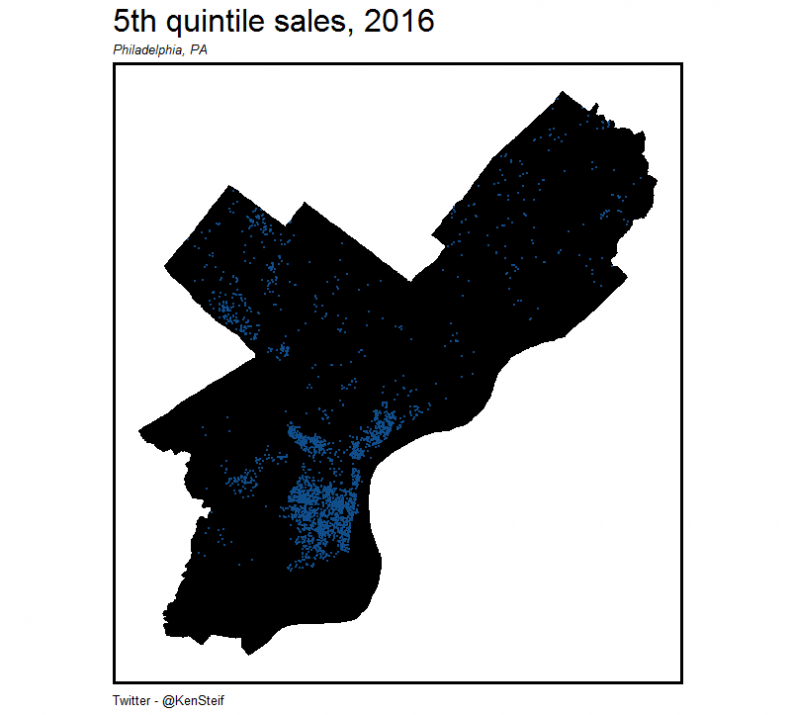
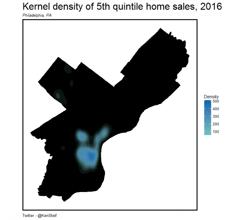
Figure 5: Density of 5th quintile sales, Philadelphia
There are far fewer sales per unit area in Northeast Philadelphia relative to central Philadelphia and when one global parameter is used to describe scale in both places, the result will be bias in one place or the other.
Most standard clustering algorithms suffer from this parameterization issue. K-means clustering, while marvelously efficient, requires the user to state an a priori number of clusters. Hierarchical clustering fares a bit better, but a single parameter is used to cut off the dendrogram.
In both instances, if the parameter is good for one neighborhood, it is likely not so good in the next.
Another clustering algorithm of note is the DBSCAN algorithm (PDF), which is expressly designed to cluster neighboring higher density points while rendering objects in lower density areas as noise.
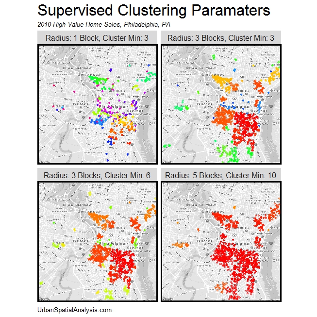
Figure 6: Four sets of DBSCAN clusters
It is not without its drawbacks however. DBSCAN has two global parameters of its own that are used to determine clustering – minimum cluster size and a maximum search radius. In practice, the heterogeneous density of sales across Philadelphia makes it difficult to specify a maximum search radius and a cluster size that can simultaneously create clusters in the dense, vertical downtown core, as well as the semi-dense rowhouse neighborhoods and those areas with detached homes.
As we can see from Figure 6, if we want University City to show up as one cluster, we have to deal with all of Center City as one cluster (lower right). If we want to find multiple clusters in Center City (top left), then most of points in University City is rendered as noise and omitted entirely.
Of course, we could fine tune these parameters by optimizing certain conditions, but at that point, why don’t we just drawn circles around the clusters we want or go back to using the neighborhood designations as above?
Thus, DBSCAN is not a generalizable algorithm that can be deployed on any dataset for any city. This is not surprising to us. Unsupervised clustering of continuous spatial data is hard.’
This experiment is one of several that we are using to track gentrification clusters over space and over time. These scale-related issues lead us to believe that the cluster approach is not the best way forward. We are however, experimenting with some novel approach for tracking real estate across the landscape like a Meteorologist tracks a storm.
Ken Steif, PhD is the founder of Urban Spatial. He is also the director of the Master of Urban Spatial Analytics program at the University of Pennsylvania. You can follow him on Twitter @KenSteif.