Urban Spatial recently had the pleasure of developing a vacant land price predictive algorithm along with a team at the Philadelphia Lank Bank – one of the most important community development institutions in Philadelphia.
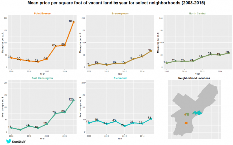
Figure 1: Mean price per square foot time series for select Philadelphia neighborhoods
Figure 1 shows that the market for vacant land in Philadelphia has exploded in recent years. Like any real estate boom, speculation plays a significant role, which poses a particular challenge when predicting prices.
By example, check out the vacant land parcel below from the rapidly changing Point Breeze neighborhood and consider why speculation makes it difficult to price this piece of land.
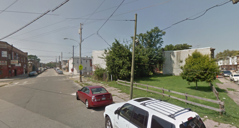
Figure 2: An example of vacant land in Point Breeze
Two discounted cash flow ninjas would likely disagree on the value of this parcel given the unbelievable price appreciation that Point Breeze has experienced (Figure 1). There is no ‘equilibrium’ price in Point Breeze currently, and no one knows how expensive land will be when the neighborhood actually stops changing.
In such a situation, oftentimes, developers will speculate and in order to model this dynamic, we have to devise a method for capturing the exuberant indecision real estate markets exhibit in rapidly changing neighborhoods.
We’ll begin with some maps and analytics and then discuss the feature engineering, model development and evaluation process. Figure 3 shows the arms length land transactions from 2008 through 2015(Q3) we use to train our models. Not surprisingly, the highest prices can be found in Center City and the neighborhoods that surround it.
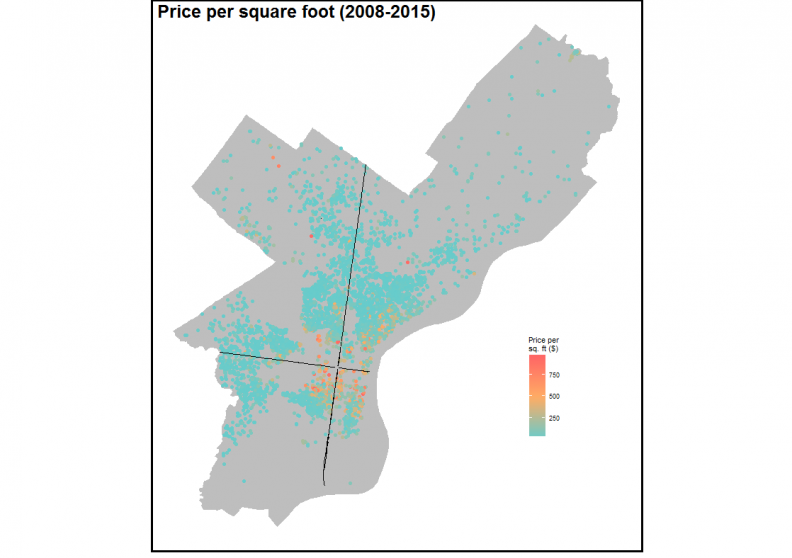
Figure 3: Price per square foot of land transactions in Philadelphia
Although the Philadelphia Land Bank has a different land disposition mechanism for higher priced parcels, we include them here because it makes the models more challenging to build (slightly different models were developed for the Land Bank).
Figure 4 below shows the Citywide vacant land price trend.
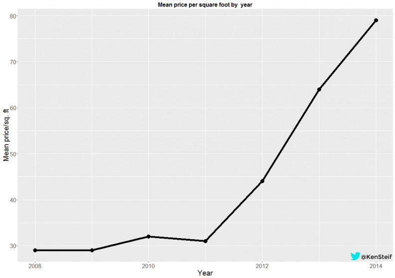
Figure 4: Mean price per square foot of land transactions in Philadelphia by year
Figure 5 shows the mean price per square foot and the number of transactions by neighborhood respectively. Although the highest prices are in and around Center City, the majority of transactions occurred in Point Breeze and many of the River Wards (Northern Liberties, Fishtown, Kensington, etc.). Not surprisingly, the historic patterns of disinvestment in Philadelphia has left these neighborhoods with the largest supply of vacant land.
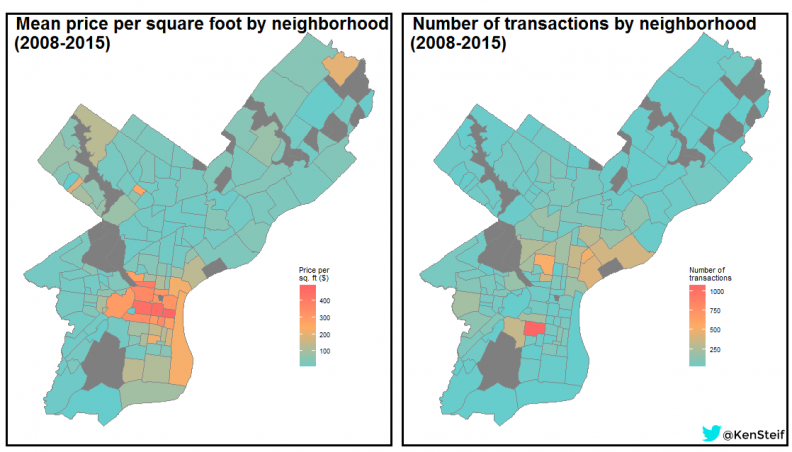
Figure 5: Mean price per square foot & count of land transactions by neighborhood
Feature engineering & modeling
Let’s revisit Figure 1 (high resolution). While the trend in Point Breeze attracts the most amount of attention, take a look at the trend in the Richmond neighborhood which illustrates the speculation issue. There is no prevailing land price in this neighborhood. Although the price trend increases between 2008 and 2015, developers in Richmond have been taken for a dizzying up/down roller coaster ride.
Figure 1: Mean price per square foot time series of select neighborhoods
We devise a series of analytics that help us capture this speculation dynamic. Ultimately, we attempt to quantify the extent to which one price observation is similar to its neighbors. Imagine the below two hypothetical neighborhoods and associated land prices illustrated as varying shades of orange.
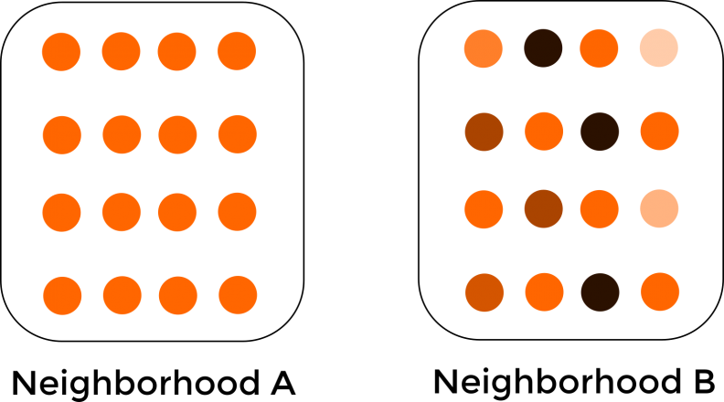
Figure 6: Two hypothetical neighborhoods and land price differences
The contrast in prices between Neighborhoods A and B are readily apparent – prices in the former are homogeneous while prices in the latter vary dramatically. Perhaps Neighborhood A is in a state of long run equilibrium while Neighborhood B is undergoing change. We see this in actual property markets – that changing neighborhoods exhibit varying prices over time because developers, buyers and sellers cannot agree the value of neighborhood amenities in the future. Capitalizing this uncertainty into land prices creates this heterogeneity.
We code these patterns by devising features using some more advanced spatial statistics and some more traditional approaches for explaining the spatial variation in price. Figure 7 illustrates some of our features. Note the first panel of Figure 7 which maps the distance to 5th quintile prices (ie. the highest prices) in the previous year for each land parcel in our training set.
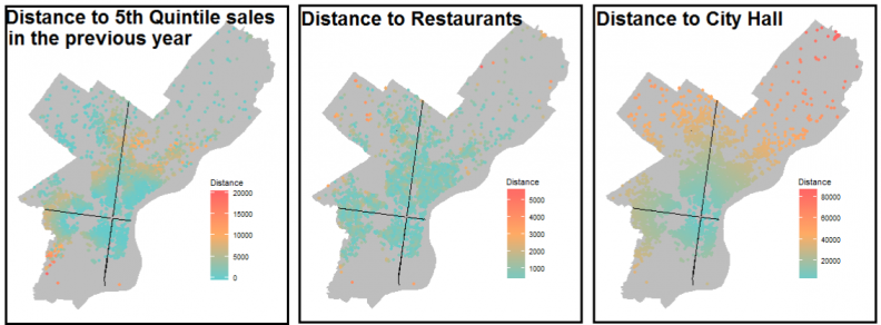
Figure 7: 3 examples of features devised for the model
The purpose of this variable is to pick up space/time dynamics by quantifying how the spatial scale of prices vary from place to place and how these dynamics can shift over time. The trick is to mine the data for these ‘endogenous’ price relationships without overfitting – which is very easy to do when predicting price as a function of nearby prices.
Like any predictive modeling exercise, our goal is to create a generalizable model that can be called upon to price land in the future.
We employ a series of feature selection techniques to ensure we don’t overfit and perform a great deal of cross-validation. To develop our models we split the dataset in half – using the first 50% of land sales to train the model and the latter 50% to test the model. This means that we can assess goodness of fit on data that the model has never seen before.
For this write-up, we display the results of a random forest model (Figure 8). The top panel of Figure 8 plots the predicted land price as a function of the actual land price. It’s clear that we predict well for land parcels that sold for $100 or less. For these parcels, the average price per square foot error is $10.21. For reference, the average observed land price per square foot in our data is $72.66. When parcels above $100 are included, the average price per square foot error is $13.97
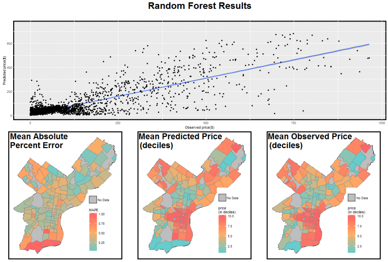
Figure 8: Random forest results
The bottom panel of Figure 8 maps the spatial extent of error. The model does a good job accounting for some of the speculation in the rapidly changing neighborhoods. Interestingly, we predict poorly in sections of the Northwest and South which may have to do with the small sample sizes in those neighborhoods (Figure 3).
Let’s take a deeper dive in to these predictions by mapping prediction errors in two changing areas of Philadelphia. Figure 9 plots prediction errors in dollars for land prices less than $100 in Point Breeze. It is clear that the model predictions become progressively worse as we move east into the rapidly changing parts of South Philadelphia.
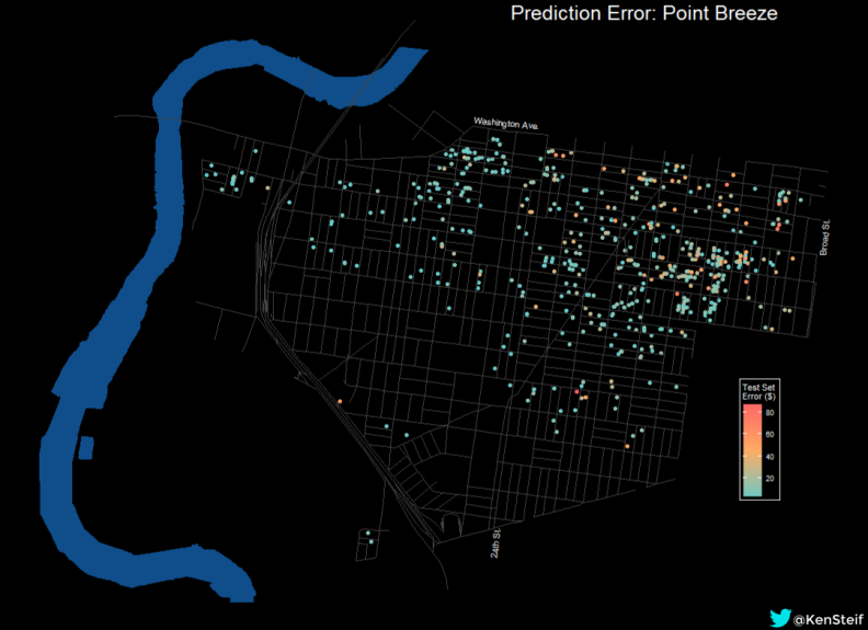
Figure 9: Prediction errors in Point Breeze
The large errors to the east are directly related to speculation and the fact that the area currently lacks an equilibrium price. Figure 10 plots prediction errors in dollars for the River Wards including Northern Liberties, Fishtown and Kensington. The same dynamic is present. As we move closer to the Delaware River, the model’s performance diminishes in the face of the unprecedented development that has occurred in these neighborhoods.
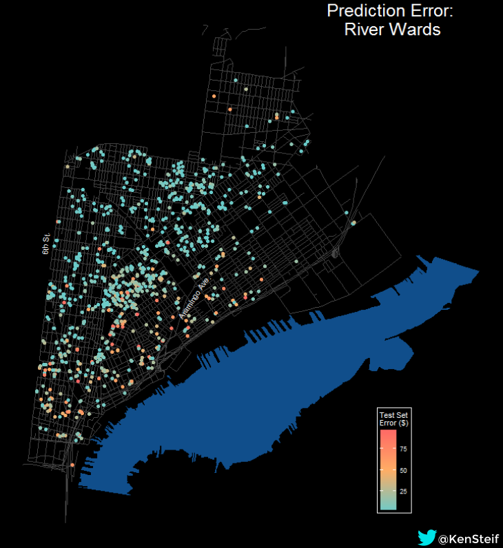
Figure 10: Prediction errors in the River Wards
Next Steps
This analysis provided a glimpse into how spatial analytics and machine learning can help predict vacant land price despite the speculation that makes land markets so volatile. While predicting vacant land price is important for the Philadelphia Land Bank’s mission – it’s low hanging fruit.
The real challenge is not to predict land value but to predict land use. After a developer purchases a piece of land or a even a property, oftentimes, they apply for a zoning variance to alter the land use. Imagine if we harnessed these past land use change experiences to predict land use for a given parcel in the Land Bank’s inventory.
This would provide a baseline land use, predicting what the market would do if it developed the property. This baseline would provide the comparison upon which alternative visions (affordable housing, community gardens, etc.) could be evaluated. For us, such an analysis would represent real innovation in how data is used for land use planning.
Ken Steif, PhD is the founder of Urban Spatial. He is also the director of the Master of Urban Spatial Analytics program at the University of Pennsylvania. You can follow him on Twitter @KenSteif