Authors:
Stacey Mosley
Ken Steif, PhD
Machine learning with spatial data is about developing more efficient ways to allocate limited resources across space.
Governments are finding new uses for the technology every day. Philadelphia is using predictive policing software to better allocate cops and Chicago is using the technology to more efficiently allocate health inspectors to potentially hazardous restaurants.
There are many other unexplored use cases and today we’re excited to present one of these – a proof of concept predicting unsafe building demolitions in Philadelphia to more efficiently prioritize building inspections.
In many post-industrial American neighborhoods, buildings and infrastructure have aged beyond their intended lifespan. In many of these places, age combined with waning market demand has left buildings under-maintained and a threat to public safety.
We believe that these historical spatial patterns can help us build powerful predictive models with the hope of detecting unsafe buildings before they deteriorate to the point of collapse.
Figure 1 below plots the 3,897 buildings that Philadelphia’s Department of Licenses and Inspections (L&I) has demolished since 2010 due to safety concerns. This number represents just 0.0073 percent of the more than half a million parcels in Philadelphia.
Note that many of the larger parcels shown in Figure 1 contained smaller buildings that were razed.
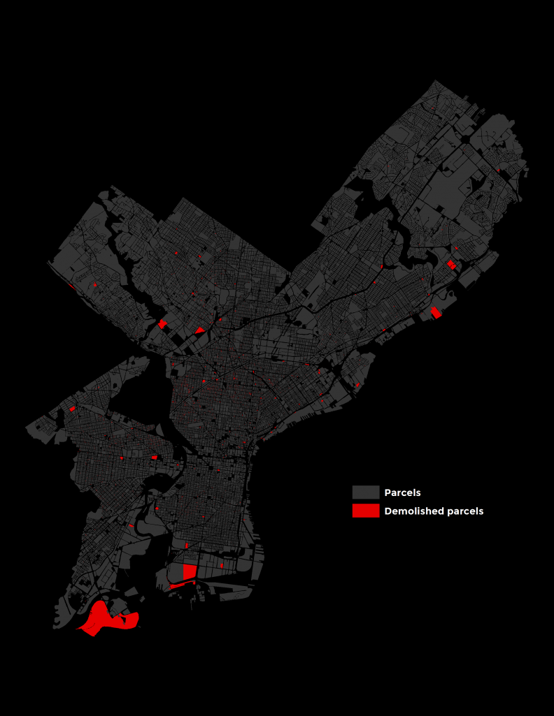
Figure 1: Locations of demolished parcels
We use these previous demolition events to train a model of demolitions and then subject that model on to the remaining parcels Citywide with the hope of predicting the probability of a building being unsafe.
Below we discuss the data used for the analysis, the models we built from the data and a conceptual design for how local governments can convert model predictions into actionable intelligence.
Data
All of the data used in the analysis are freely available for download via OpenDataPhilly and Philadelphia’s very robust open data APIs.
We implement our hypothesis about how spatial and historical trends can help predict building safety by measuring the distance from each parcel to a series of environmental factors including building inspection outcomes, crime, vacancy, 311 data, real estate values and several parcel specific indicators as well.
Figure 2 maps three of these indicators.
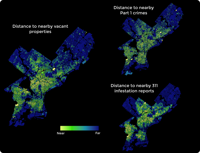
Figure 2: 3 variables used as predictors
Methodology
The goal of these preliminary models is to estimate the probability that a given building might be unsafe.
There are two ways to do this. The first is to collect lots of data; put it all on the same scale and then ask a building inspector to tell us, based on experience, how each factor should be weighted. We could then overlay each of these scaled factors into one ‘building safety index’.
The second strategy is to subject the same data to a statistical model which is able to fit the weights specifically according to how well the data explains actual building demolition events.
The difference is not trivial. Although the inspector’s experience is invaluable, machine learning algorithms can search for patterns and investigate countless hypotheses with greater efficiency and accuracy than a human being.
To avoid overfitting, we develop our model on a ‘training set’ that uses just 5% of the more than 530,000 parcels citywide (n=26,517). The remaining 95% is set aside as the ‘test set’.
A more parsimonious dataset is created by running our data through both stepwise logistic regression and recursive feature elimination.
We then estimate models using four separate classifier algorithms: logistic regression, naïve bayes, random forests and gradient boosting machines.
Several models are estimated for each classifier followed by an examination of each model’s goodness of fit.
Although we are using these ‘classification’ models to predict a discrete outcome (building demolitions), the predictive outcome of interest is actually a continuous metric – the ‘predicted probability’ that a building is unsafe.
Results
To begin, we examine Receiver Operating Curves (ROC) for each model. ROC curves are one indication of how well a classifier model fits the actual data. They tell us the tradeoff between the true positive rate (the proportion of actual building demolitions that the model correctly predicts) and the true negative rate (the proportion of actual non-demolitions the model predicts).
Figure 3 illustrates ROC curves for our four model types. Here we are predicting for the test set using the 5% random sample training set. While there is some comparability across the four models, the random forest and GBM specifications (each with an area under the curve of around 0.91) stand out.
It is worthy to note that the logistic regression is relatively powerful in this context.
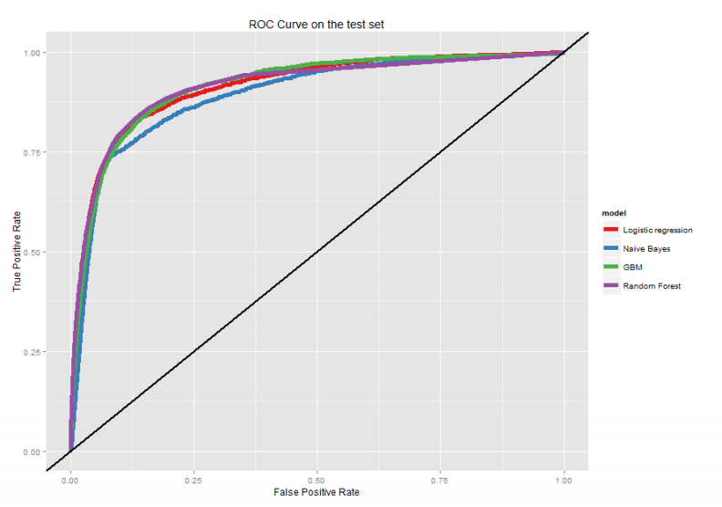
Figure 3: ROC Curves for the four predictive algorithms
For each classifier, we compared the properties predicted to be demolished to those that were actually demolished for the test set. Our accuracy was relatively high for each model type but the GBM and random forest models performed better.
Turning to the predicted probabilities, given that most of the buildings in Philadelphia are relatively safe, our expectation is that the predicted probabilities, on average, should be quite small. Figure 4 illustrates a histogram of predicted probabilities for each model. Here, we show only the count of buildings citywide with a probability of 5% or less that they are unsafe.
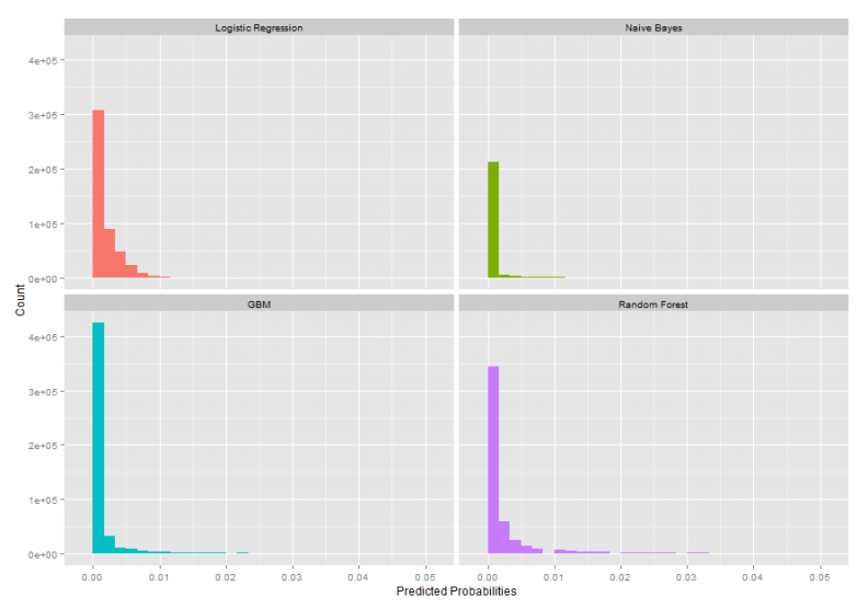
Figure 4: Histogram of predicted probabilities for each predictive algorithm
Ultimately, we selected the GBM model based on its relative goodness of fit, how well it classified on the test set as well the conservative number of parcels it predicts as being unsafe.
Our final model finds about 1,800 parcels citywide with the predicted probability of an unsafe outcome being greater than 10%. As of the time of this analysis, 365 of these have not been inspected since 2007. The most common zoning types are as follows:
RSA-5 (Dense single family) – 917
RM-1 (Lower density multi-family) – 758
CMX-2 (Commercial mixed use) – 79
RSA-3 (Medium density single family) – 41
I-2 (Medium industrial) – 12
Figure 5 plots those parcels with predicted probabilities greater than 10%. Note the underlying choropleth map which shows the total number of these parcels by census tract.
Figure 5: Map of predicted probabilities
Next steps
Figure 6 shows what an inspector-facing mapping application might look like. The purpose is to use the predicted probabilities from the model to help prioritize inspections. Here we refer to the probability of an unsafe outcome as a ‘safety predictive score’.
This hypothetical tool could be used by inspectors to visit properties while on a pre-assigned route or to help generate daily inspection routes. The tool could also geo-locate the inspector’s current location and return results for those in the immediate surroundings.
By accessing additional parcel and block-level open data, we can provide inspectors with a range of metrics to make the decision-making process more efficient and more informed.
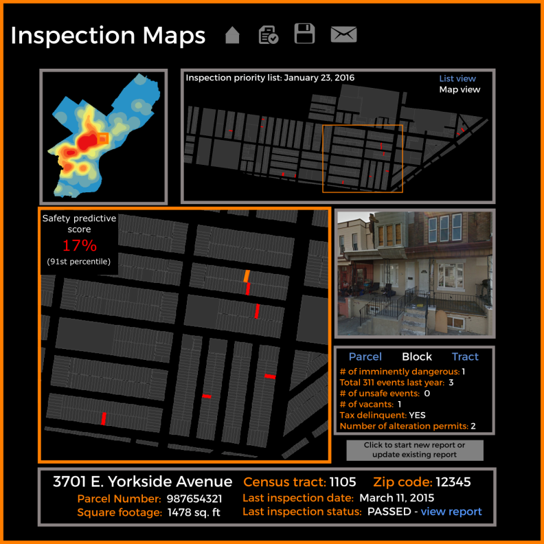
Figure 6: A mock-up of a building inspection app using the predicted probabilities.
Conclusions
In this proof of concept we developed a model of unsafe building demolitions with the hope of using the resulting predicted probabilities to help prioritize building inspections.
The models we developed were robust, but they could certainly be improved. The greatest concern is that our current models are overfit on the disproportional number of spatial variables we input. Ideally we’d like to gather more parcel level indicators and spend more time performing feature selection and model tuning.
Nevertheless, it’s clear that the prioritization of building inspections is an important use case for extending machine learning in to government.