Earlier this semester, my students learned how to build spatial predictive models. For their final projects, they attempted to use machine learning to predict across both space and time – a proposition that is risky, at best.
No one has a crystal ball and any major exogenous shock (like a recession) could render the past a poor predictor of the future.
For this exercise, the goal was to use data from 1990, 2000 & 2010 to predict urban land cover in 2020.
Why would we want to predict urban development? Visioning is an important component of city planning. The goal is to best allocate our resources today where they will be most needed in the future. Prediction lends itself nicely to this goal.
Our motivation is to harness the space/time trend behind urban development and test to what extent this trend is applicable for the future.
Figure 1 shows the extent of our study area – 11 counties in 3 states in and around Philadelphia.
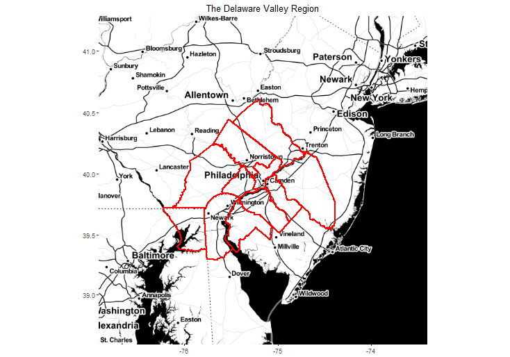
Figure 1: The Delaware Valley Region
We begin with land cover data classified from satellite imagery. These data are then joined to census tracts.
To get a sense of how our region grew since 1990, Figure 2 shows the spatial extent of urban development by tract as a percent of total land area between 1990 and 2010.
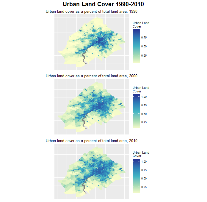
Figure 2: Urban Land Cover 1990-2010
Growth really exploded across the region between 1990 and 2000. Below is the same trend broken out by county.
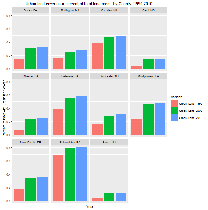
Figure 3: Urban Land Cover 1990-2010 (bar chart)
As a precursor to predicting for 2020, we’re going to test the extent to which our data allows us to predict for 2010 (a year we have actual data for). If we can develop a generalizable model for 2010, it may be reasonable to use it for 2020.
To get a better sense of where most changes occurred, Figure 4 shows the change in urban land cover between 2000 and 2010. Most of the development appears to have happened outside of Philadelphia, in the suburbs.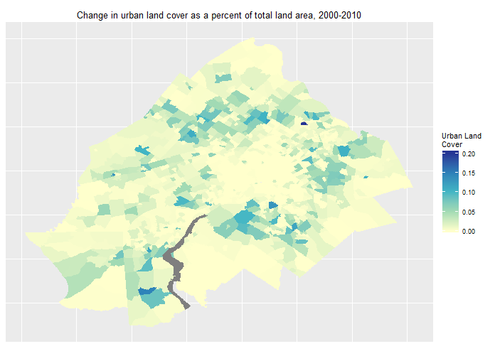
Figure 4: Percent change in Urban Land Cover 2000-2010
A large number of independent variables were compiled for this analysis. Many came from the U.S. Census but some were generated explicitly for the purpose of predicting across space and time. Figure 5 shows four selected variables.
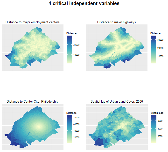
Figure 5: Selected independent variables
The last variable, the ‘spatial lag’ of urban development, is worth discussing in a bit more detail. Typically, urban development does not happen in the middle of a cornfield. Developers rely on preexisting infrastructure like roads and schools.
Thus we hypothesize that growth in 2010 is in part, a function of nearby growth in previous time periods. We develop a series ‘space/time lags’ as pictured in Figure 5 to quantify this feature of the urban landscape. Figure 6 shows the statistical relationship between census tract urban development in 2010 and the average development in 2000 of surrounding tracts.
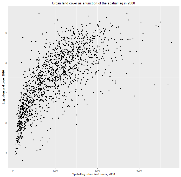
Figure 6: The spatial lag predictor
Growth begets growth and thus we should expect a strong statistical relationship between urban development in 2010 and nearby growth in 2000.
This approach, while powerful, is also very risky if our goal is to develop a generalizable model that predicts for 2020. If the model is overfit on these previous space/time trends then it is unlikely to predict well for the next time period.
Here the threat of overfitting is overcome by way of a some creative model stacking – using predictions from previous models to inform our final model. I wish I could say more, but that would ruin it for next year’s class!
So how well does our model do?
Cross-validation is used to train the model. Here the model is tested on a random subset of the data, goodness of fit metrics are calculated, the subset is shuffled back into the dataset, a new subset is generated and the model is tested again.
This process is repeated over and again until we get a sense whether our model performs consistently regardless of the data it’s tested on or whether it’s sensitive to trends in the model that we may have omitted. The goodness of fit across hundreds of cross-validation subsets varies less than 1% suggesting that our model is flexible.
Overall, the mean absolute percentage error is just 2.8%.
Of course, it is not just random subsets that are important for judging how suitable our model is. We also want to ensure that it is sensitive to different urban contexts as well. By example a model that predicts well in Philadelphia but not so well in a suburban or rural county is clearly not generalizable.
Thus, we also wish to test how well the model performs for different counties.
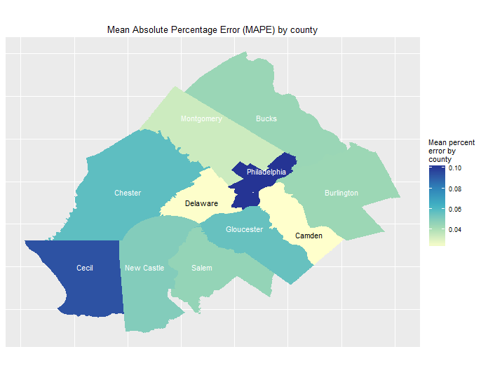 Figure 7: Mean absolute percentage error by county
To do so, the model is estimated for all counties except one, and then tested on the hold out county. A goodness of fit metric is calculated – in this case the mean absolute percentage error. That county is then shuffled back into the data, a new one is withheld, the model is re-estimated and then tested on the hold out. This process continues until each county has had a turn being withheld.
Figure 7 maps the results. The first thing to notice is that at most, the models errs no more than 10% on average – and that’s just for two counties. Most interesting is that these two counties are Philadelphia, far and away the biggest city in the study area, and Cecil County Md. Google Earth shows us just how rural this county is.
Thus, if the model is performing equally as poorly (and 10% error is pretty good) in a very urban and a very rural county, then we can conclude that it’s well generalizable.
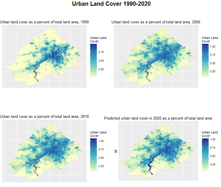
Figure 8: Urban land cover 1990-2020 (2020 predictions)
The final step then is to predict for 2020 (Figure 8). To get a better sense of the decennial growth by county, check out Figure 9.
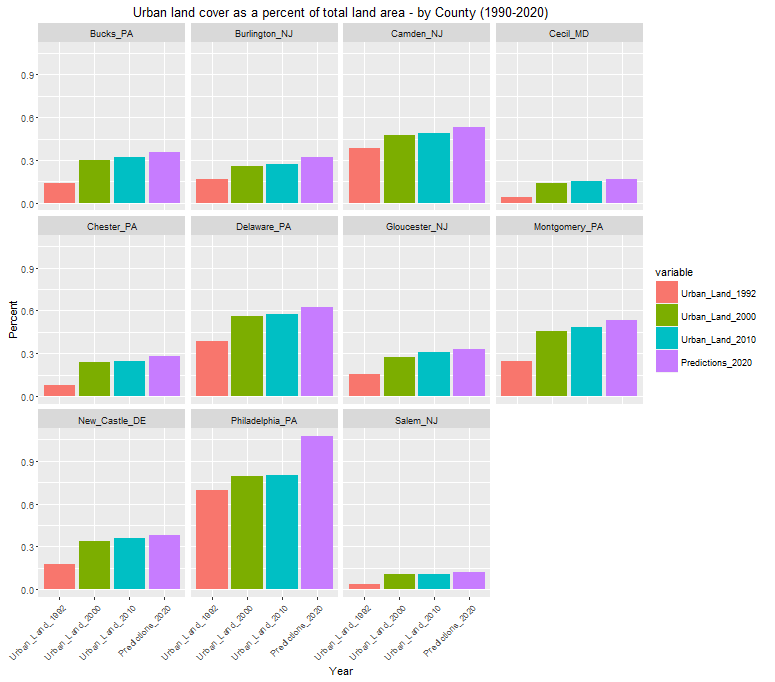
Figure 9: Urban land cover 1990-2020 (2020 predictions) – bar plot
The model tells us that we should expect all counties to grow but that some should grow faster than others. The model predicts the biggest growth in Philadelphia, which is not hard to believe if you’ve witnessed, as I have, the explosive building boom that the City has experienced in recent years.
Check out this graph from Pew Charitable Trusts that show the growth in Philadelphia building permit activity up until 2014.
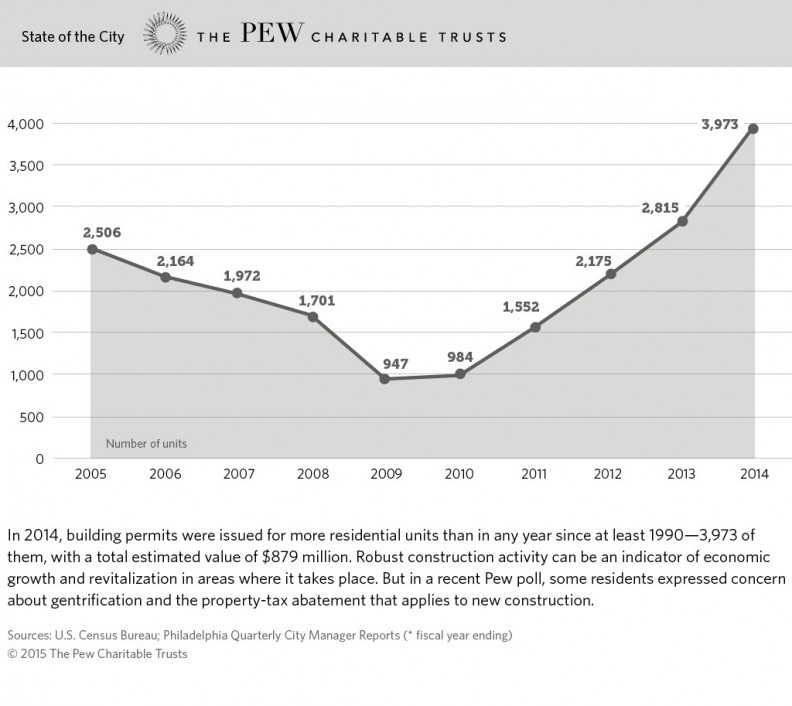
The model clearly predicts that predominately urbanized counties will grow the most. This may be true or it may that the model is biased to believe it so. I already told you that the model is has been explicitly trained to believe that “growth begets growth”. Of course, this is what is so difficult about forecasting. The best we can do is to train the model on what happened already and cross our fingers that the trend continues.
This is not always true of course. My favorite visual evidence of this comes from the 1925 Plan for Cincinnati. I’ve taken the original historical plot of predicted population growth and augmented it with the actual population through 2010.
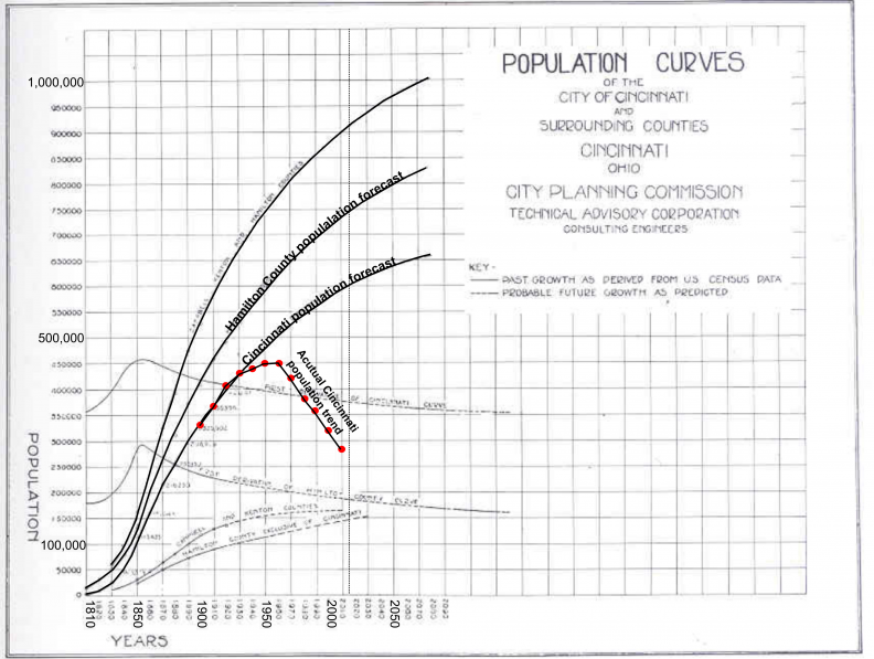
When the Plan’s authors were making predictions for next several generations, they had no reason to assume that their industrial and transportation powerhouse of a city would not continue to thrive. Like many cities of it’s time however, Cincinnati fell victim to seismic macro-economic shifts including deindustrialization.
Statistically speaking, our urban growth model presented above works well. However, if I traveled back to 1925 and gave the architects of Cincinnati’s plan a laptop running R, their model might also appear robust.
Nevertheless, building growth models is still an important part of the visioning process. If we believe in policies that protect open space, promote sustainable forms of transportation and the like, then forecasting growth in to the near future can help us make better budgeting, legislative, design and engineering decisions today.
Want to learn how to build these models and others? Check out the Master of Urban Spatial Analytics at Penn where I currently teach. Check me out on Twitter, @KenSteif.
