Suitability modeling is one of the most important GIS skill sets for a spatial analyst to master. Traditionally, site suitability is done using raster GIS but for this post, I’d like to offer a contrasting methodology that is a bit more statistical in nature.
For this example, I’m going to try to locate land in Pennsylvania that is suitable for preservation using open data from PASDA .
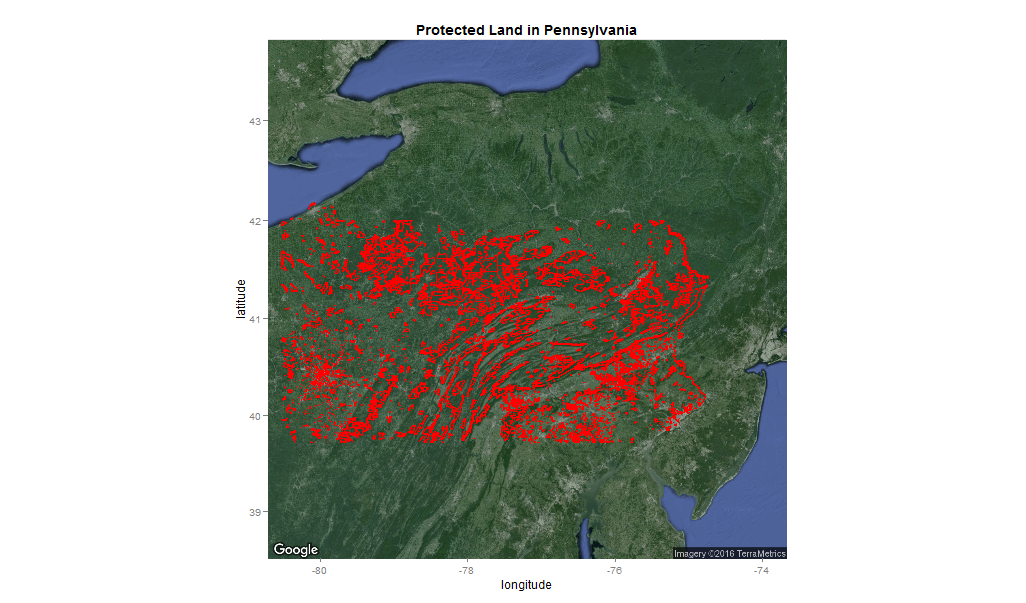
Figure 1: Preserved land in Pennsylvania
The raster approach
Imagine that in an effort to site more preserve land in Pennsylvania, we put together a panel of preeminent ecologists, city planners and naturalists and asked them suggest some spatial ‘decision factors’ that they believe are important for targeting conservation.
Suppose these experts suggested the four factors as illustrated in Figure 2. They are areas close to rivers; close to steep slopes; far from cities and of higher elevation.
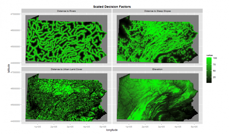
Figure 2: Preserved land decision factors
Each of the four decision factors illustrated in Figure 2 have been scaled from 1 – 100 which allows them to be overlaid into a site suitability map (Figure 3).
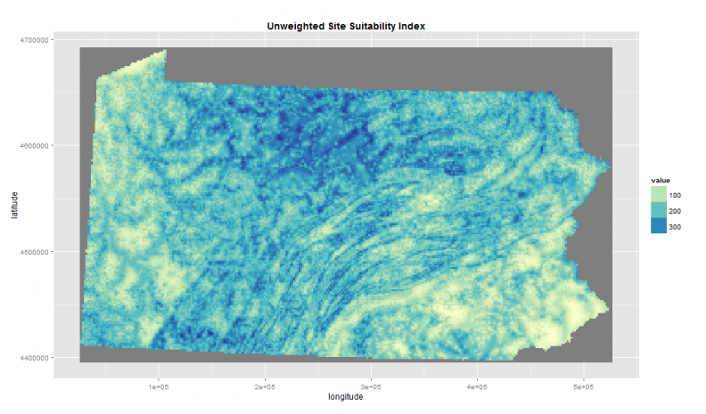
Figure 3: Unweighted site suitability overlay
Notice that the highest site suitability score in Figure 3 is ‘400’, representing areas that score ‘100’ on all four decision factors.
Next, let’s imagine that we then go back to our land conservation experts who inform us that in their experience, distance to rivers isn’t nearly as important as the other factors. In fact, their preference is to weight the site suitability index as such:
Distance to Rivers + Distance to Urban Areas + (Distance to steep slopes * 3) + (Elevation * 2)
Figure 4 presents the output of this ‘map algebra‘ statement.
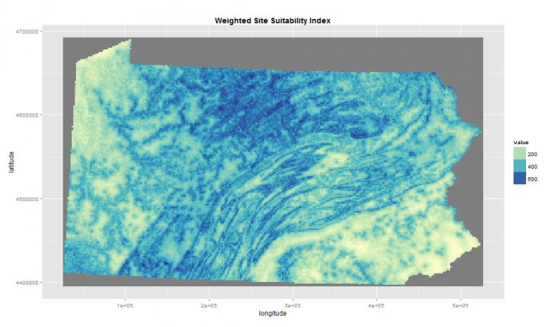
Figure 4: Weighted site suitability overlay
Notice that less emphasis is put on the rivers in Figure 4, but according to the weighted overlay much of the state is ripe for conservation. Of course, we could continue to adjust the weights until we have an acceptable suitability surface.
The predictive approach
What’s interesting about protected land as an outcome, is that it is the product of so many human-level interactions. The forces that lead to actual protection are so much more complicated than just these demand-side, decision factors.
The actual ground-truthed outcome of preservation embodies many social, economic and political dynamics.
As such, the best way to judge the suitability of protected land is to try and model the spatial forces that underlie the actual preservation outcome.
If this can be done reasonably well, the resulting spatial predictions can be thought of as a measure of suitability.
To begin, we generate a vector “fishnet” to quickly sample our raster data into a vector format which can then be brought into a statistical software like R (Figure 5).
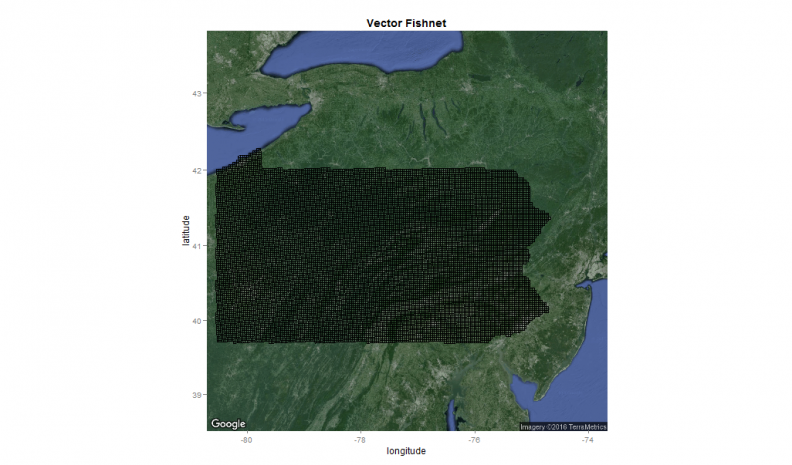
Figure 5: A 3000m vector fishnet
The fishnet is comprised of grid cell polygons which mimic the raster format. At 3000m by 3000m however, these grid cells represent the data at a pretty low spatial resolution which will help keep the dataset small (n = ~13k) and allow for faster processing.
Great attention is paid to not overfitting the model in order to ensure that the model returns some areas as suitable that aren’t already protected.
The data is split into a 50% training set which is used to estimate a binary logistic regression model. Figure 6 displays the results.
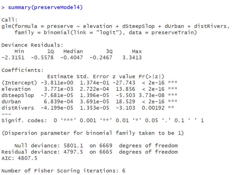
Figure 6: The logistic regression
Although we’re not particularly interested in the coefficients, they tell us for instance, that on average, the farther we get from urban areas the greater the probability that land has been preserved. What we are interested in is the model’s predicted probabilities.
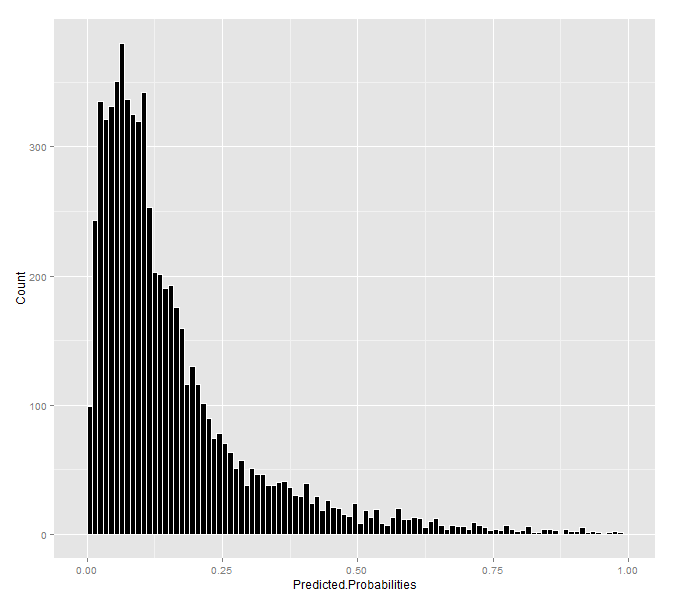
Figure 7: Histogram of predicted probabilities
Figure 7 shows that most of the predicted probabilities are low, suggesting much of the state is not suitable for preservation. What do these probabilities look like spatially?
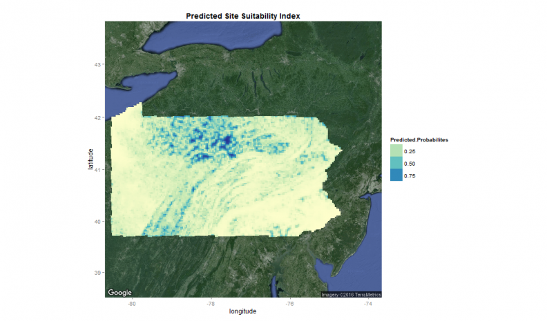
Figure 8: Spatial distribution of predicted probabilities
The higher the probability the more suitable the land is for protection, as least as our simple model predicts it. It is worth noting that compared to the weighted overlay, the statistical model makes much more conservative estimates about which areas are suitable for protection.
Figure 9 overlays development land cover and current protected lands atop these probabilities.
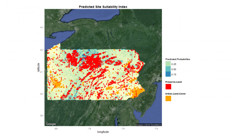
Figure 9: Spatial distribution of predicted probabilities with overlays
If we were to replicate this model in real life, we’d want to gather many more variables that can account for a host of different spatial and aspatial phenomena. Perhaps something like county-level fixed effects might help account for local differences in land use or conservation policy.
Again, I think the real value of the predictive approach relative to the traditional raster overlay is that the statistical model provides a suitability metric that considers land that has actually been preserved in the past.
I’ve made the argument in the past that although the experience of domain experts is invaluable, allowing a model to uncover the important underlying relationships behind a given outcome (the ‘weights’) is likely a better formula for deciding where to allocate limited resources.